Machine Learning Model Evaluation

  

What exactly is Machine Learning?

Machine Learning is a hot topic in information technology right now. Machine Learning enables our computer to gain insight from data and experience in the same way that a human would. Programmers teach the computer how to use its past experiences with various entities to perform better in future scenarios in Machine Learning.

Machine Learning entails creating mathematical models to assist us in understanding the data at hand. Once fitted to previously observed data, these models can be used to predict newly observed data.

Models in Machine Learning are only as useful as their predictive power; thus, our fundamental goal is not to create models but to create high-quality models with promising predictive power.

Binary Classifier Predictions Evaluation

Accuracy is a well-known performance metric used to distinguish a strong classification model from a weak classification model when evaluating a Binary Classifier. Simply put, accuracy is the total proportion of correctly predicted observations. The mathematical formula for calculating Accuracy has four (4) main components, namely TP, TN, FP, and FN, and these components allow us to investigate other ML Model Evaluation Metrics. The following is the formula for calculating accuracy:

Where:

• TP stands for the number of True Positives. This is the total number of observations that fall into the positive category and were correctly predicted.

• TN is the number of True Negatives. This is the total number of observations that fall into the negative category and were correctly predicted.

• The number of False Positives is denoted by FP. It is also referred to as a Type 1 Error. This is the total number of observations that were predicted to be in the positive class but ended up in the negative class.

• The number of False Negatives is denoted by FN. It is sometimes referred to as a Type 2 Error. This is the total number of observations that were predicted to be in the negative class but ended up in the positive class.

The main reason people use the Accuracy Evaluation Metric is because it is simple to use. This Evaluation Metric takes a straightforward approach and explanation. As previously stated, it is simply the total proportion (total number) of correctly predicted observations. Accuracy, on the other hand, is an Evaluation Metric that does not perform well in the presence of imbalanced classes-when the Accuracy value is high but the model lacks predictive power and most, if not all, predictions are going to be incorrect.

For the reasons stated above, when we are unable to use the Accuracy Evaluation Metric, we must resort to other evaluation metrics in the scikit-learn arsenal. These include, but are not limited to, the evaluation metrics listed below:

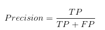
Precision

This is the proportion (total number) of all observations that were predicted to be positive and are actually positive. The Precision Evaluation Metric formula is as follows:

Recall

This is the proportion of observations predicted to be in the positive category that are actually in the positive category. It indirectly indicates the model's ability to identify an observation that belongs to the positive class at random. The Recall formula is as follows:

F1 Score

This is an averaging Evaluation Metric that produces a ratio. The Harmonic Mean of the precision and recall Evaluation Metrics is another name for the F1 Score. This Evaluation Metric is a measure of our model's overall correctness in a positive prediction environment—that is, how many of the observations that our model labelled as positive are actually positive. The F1 Score Evaluation Metric has the following formula:

Analyzing predictions from multiclass classifiers.

All input data in Machine Learning is not balanced, which leads to the problem of Imbalanced Classes. With the Accuracy Evaluation Metric out of the picture, we focus on Precision, Recall, and F1 Scores. In Python, we use parameter options to aggregate the evaluation values by averaging them. The three primary options available to us are:

macro - We tell the compiler to compute the mean of the metric scores for each class in the dataset, weighting each class equally.

Weighted - We calculate the mean of the metric scores for each class and weight each class directly proportional to its size in the dataset.

micro - In this section, we compute the mean of the metric scores for each OBSERVATION in the dataset.

Visualizing the Performance of a Classifier

A Confusion Matrix is currently the most popular way to visualize a classifier's performance. A Confusion Matrix is also known as an Error Matrix. A Confusion Matrix is extremely interpretable. It consists of a simple tabular format that is frequently generated and visualized as a Heatmap. The predicted classes are represented by each column of the Confusion Matrix, while the true (or actual) classes are represented by each row.

There are three critical facts to understand about a Confusion Matrix:

• A Perfect Confusion Matrix will have values along the main diagonal (from left to right) and zeroes (0) everywhere else.

• A Confusion Matrix shows us not only where the Machine Learning Model went wrong, but also how it arrived at those conclusions.

• A Confusion Matrix can work with any number of classes; for example, having a dataset with 50 classes has no effect on model performance or the Confusion Matrix; it simply means your Visualized Matrix will be very large in size.

Evaluating the Performance of a Regression Model.

MSE is one of the most commonly used and well-known Evaluation Metrics for a Regressor. MSE is an abbreviation for Mean Squared Error. MSE is calculated as follows in a mathematical representation:

Where:

• The number n denotes the number of observations in the dataset.

• Yi is the true value of the target value for observation that we are attempting to predict. I. 

• Yi is the predicted value of Yi by the model.

The squared sum of all the distances between predicted and true values is used to calculate MSE. The greater the MSE output value, the greater the sum of squared error in the model, and thus the poorer the quality of model predictions. As shown in the model, there are benefits to squaring the error margins:

• To begin, squaring the error forces all error values to be positive.

• Second, this means that the model will penalise a few large error values more than many small error values.